Marshall and Olkin [1] proposed a way of introducing a parameter in a family of distributions to compete with such commonly used distributions as the Weibull, gamma and lognormal distributions. Let G and g be the cumulative distribution function (cdf) and the probability density function (pdf) respectively, indexed by the vector of parameter λ∈Λ. The pdf of the Marshall-Olkin extended model is given byf(x;α,λ)=αg(x;λ){1−α¯¯G¯¯¯(x;λ)}2,x∈X,α>0,λ∈Λ,(1)where X is the sample space defined for g and G, G¯¯¯=1−G and α¯¯=1−α. Henceforth, we use the notation X∼MOEg(α,λ) to refer to a random variable with density provided in (1). Marshall and Olkin [2] called α the “tilt” parameter because the hazard rate of MOEg(α,λ) is shifted below (α≥1) or above (0<α≤1) the baseline hazard rate related to g. Castellares and Lemonte [3] also showed an interpretation of MOEg(α,λ) based on the distribution of order statistics. Specifically, let {Xn,n∈N} be a sequence of independent, identically distributed (iid) random variables in which each Xn has baseline cumulative function G. Also, let N1∼Geo(α), for 0<α<1 and N2∼Geo(α−1), for α>1, with Geo(p) denoting the geometric distribution with mean 1/p. We have that{YN1=min(X1,…,XN1)∼MOEg(α,λ),ZN2=max(X1,…,XN2)∼MOEg(α,λ),if0<α≤1,andifα>1.In their initial work, the authors considered the case where G and g came from the exponential and Weibull models. Other recent proposals discussed in the literature include the Pareto [4], extended Weibull [5], gamma [6], Lomax [7], linear failure-rate [8], Burr type XII [9], normal [10], geometric [11], Birnbaum-Saunders [12], extended Weibull [13,14], modified Weibull [15], beta [16], generalized exponential [17], extended generalized Lindley [18], additive Weibull [19], Kappa [20] and logistic-exponential [21] distributions, among others. [22] presented a generalization based on the exponentiated method discussed in [23], named the Marshall-Olkin generalized-G family, which included as a particular case the Marshall-Olkin extended model in [1].From a statistical point of view, interpretations for some of those extensions are as follows: for α≥1, Marshall and Olkin [1] interpreted the Marshall-Olkin extended exponential model as the conditional distribution, given the variable in the positive axis, of a random variable with logistic survival function. Ristic et al. [6] interpreted the Marshall-Olkin extended gamma model as a minification process, useful in a time series context. Ghitany et al. [7] interpreted the Marshall-Olkin extended Lomax model as a compounding process with exponential mixing model. A similar interpretation was presented in Ghitany and Kotz [8] for the Marshall-Olkin extended linear failure-rate. Gómez-Déniz [11] discretize the Marshall-Olkin extended exponential model in Marshall and Olkin [1] to obtain a generalized version of the geometric distribution. This model also can be seen as an infinite mixture of geometric distributions.Applications to real data sets for some of those extensions include remission times in bladder cancer patients [7] and cancers in general [24], reliability analyses of electronic devices [15] and mechanical components [20], stress-rupture life of kevlar 49/epoxy strands [25], strengths of glass fibers [25], solid epoxy electrical-insulation in an accelerated voltage life test [25], flood peaks in a river [21], lifetimes of front disk brake pads [21], annual salaries of baseball players in Major League Baseball [26], stream flow amounts [20], etc.We note that in many simulation studies presented in those works, the bias for the estimator of α is greater than the bias for the estimator of λ (the vector for the baseline model). If the estimators are biased, this implies that they are inconsistent; consequently, any function of these estimators will be inconsistent. In particular, any measurement of interest, such as mean, median, quantile, etc. will be inconsistent.For illustrative purposes, we considered the Marshall-Olkin extended exponential (MOEE) with pdf given byf(x;α,θ)=αθe−θx(1−α¯¯e−θx)2,x>0,α>0,θ>0,(2)and the the Marshall-Olkin extended Rayleigh (MOER), a submodel in the class proposed by Alshangiti et al. [15], for which pdf isf(x;α,θ)=2αθxe−θx2(1−α¯¯e−θx2)2,x>0,α>0,θ>0.(3)Note that in both models, the dimension of λ is 1. Moreover, λ=θ. Figure 1 shows the density plot for different choices of α and θ in MOEE and MOER models, respectively.

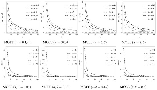
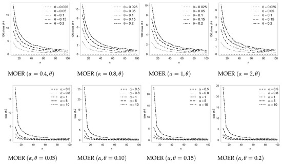
Figure 1. Pdf for MOEE and MOER models under different combinations of parameters.Figure 2 and Figure 3 show the estimated bias based on 5000 replicates for the MOEE and MOER models and different sample sizes for the maximum likelihood estimators (MLE). These figures illustrate that the bias for the estimator of α is considerably greater (in relative terms) than the bias of θ in the same models. For this reason, we propose to study a methodology to reduce the bias for the MLE of α in the general class of model defined in (1), which can be applied to any member of the class, i.e., with any considered g and G in the baseline model.

Figure 2. Estimated bias for the MLE of α and θ in the MOEE(α, θ) under different scenarios based on 5000 replicates.

Figure 3. Estimated bias for the MLE of α and θ in the MOER(α, θ) under different scenarios based on 5000 replicates.In a frequentist context, in general, the maximum likelihood method is used to estimate the parameters of the model. The inferences depend strongly on asymptotic properties of the MLE, for instance, let αˆ be the MLE of α. Among these properties, we have that the MLE is approximately non-biased, i.e., E(αˆ−α)=0 and follows a normal distribution when the sample size is large enough. However, likelihood inferences based on asymptotic approximation, when samples are of small or moderate size, may not be reliable.The study of the behavior of the bias of MLE in small samples is an important area of research. There are several works in the literature related with bias correction; they can be divided into two main approaches: the corrective and the preventive, proposed by Cox and Snell [27] and Firth [28], respectively. In the first method, the bias is corrected after the MLE calculation; in the second, with a modification in the score function, the procedure already computes a less biased estimator than the regular MLE. The two methods are comparable, however Firth’s procedure has gained more popularity in recent years. Assuming g free of parameters in MOEg(α,λ), the aim of our paper is to obtain, through the preventive method, a bias-corrected maximum likelihood estimator (BCE) for α that is less biased and shows the useful side-effect for MLE for the components of the vector λ.The work is organized as follows. In Section 2 we develop the procedure to estimate a bias-corrected parameter in MOEg(α,λ). Monte Carlo simulation experiments are presented in Section 3 to discuss the importance of the expression obtained in the previous section, which produces much less biased estimates than the traditional procedure. In Section 4, we consider two empirical examples. We conclude in Section 5 with some final remarks. In the Appendix A we present details of the quantities needed in our work.
https://www.mdpi.com/2073-8994/12/5/851/htm
Diego I. Gallardo, Osvaldo Venegas, Tiago M. Magalhães, Yolanda M. Gómez

